Lab 02 - Familiarization With ArcGIS Desktop DEM Raster Tools and ArcScene

Introduction

The goal of this Field Methods lab activity was to familiarize us with the various spatial analysis tools that are commonly used on DEM raster files in ArcGIS desktop applications.  Understanding what each of these common tools does and the products that will be created upon running these tools was also an important goal of this lab.  Finally, another goal was to gain experience in the viewing of DEM raster data in a 3D platform such as ArcScene

Methods

To begin this lab, provided DEM data was copied into our individual class folders.  This data, had it not been provided for us, was obtainable through the WI DNR or through the USGS.  With this data, we opened ArcGIS desktop and created a file geodatabase to house the data in each of our individual folders.  With this done, the final step before processing the data was to turn on the Spatial Analyst extension under the Customize menu to allow for the use of Spatial Analyst tools.

With these set up steps complete, the first tool to be run was the Contour Tool found under Spatial Analyst>Surface>Contour.  This too creates contour lines at a user set interval, in this case 10 meters, and exports the output as a layer that can be added to a map document.

Figure 1. 10 meter contour interval of Eau Claire County DEM

The next Spatial Analysis tool to be run was the slope tool, found under Spatial Analyst>Surface>Slope.  This tool creates a raster file showing the relative steepness of slopes based off an input DEM.

Figure 2. Slopes of Eau Claire County DEM

The next tool after slope was the aspect tool, found under found under Spatial Analyst>Surface>Aspect.  This tool determines the aspect, or the cardinal direction, that each slope faces.

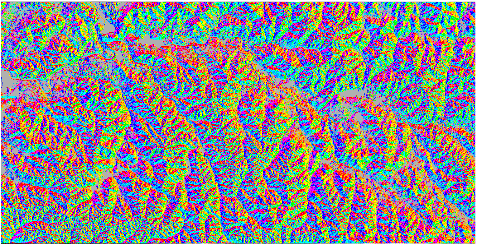
Figure 3. Slope Aspect of Eau Claire County DEM

The final Spatial Analysis tool to be run on this DEM is the Hillshade tool, found under Spatial Analyst>Surface>Hillshade.  This tool creates a shaded relief of a DEM that allows for better visualization of the topography of an area.

Figure 4. Hillshade of Eau Claire County DEM

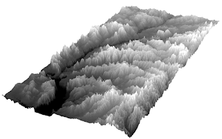
Once all of the Spatial Analysis tools had been run, the next step was to visualize the DEM in ArcScene.  This was done to express the DEM in all three dimensions rather than in 2D like in ArcGIS desktop.  To do this, the DEM was set to 'floating on a custom surface' either by meters to feet, feet to meters, or based on a custom value.  These values determined the overall vertical exaggeration of the DEM.

Figure 5. Eau Claire County DEM shown with different levels of vertical exaggeration.

Discussion

This lab was very straight forward, with simple easy to understand directions that guided us students through the lab to accomplish the goals of the exercise.  

Conclusion

Overall this lab was very useful in developing my understanding of some of the spatial analyst tools present in ArcGIS desktop. this lab was also great in allowing us to gain more experience in working with DEM's both in ArcGIS desktop and ArcScene as well.

Evaluation

1.     Prior to this activity, how would you rank yourself in knowledge about the topic. 

         4-A good amount of knowledge

2.       Following this activity, how would you rate the amount of knowledge you have on the topic

         5- I am an expert)

3.       Did the hands-on approach to this activity add to how much you were able to learn.

         4-Agree

4.       What types of learning strategies would you recommend to make the activity even better?

          More in depth use of these spatial tools for a wider variety of applications.

Lab 1 - Creation of a Digital Elevation Surface using critical thinking skills and improvised survey techniques

Introduction

                The goal of the first Geospatial Field Methods lab activity was to collect the data to be used in the creation of a digital elevation surface to be created in a later lab exercise. This was accomplished using a variety of survey tools and sand boxes with pre laid out grids located on the eastern side of Phillips Science Hall on the lower portion of the University of Wisconsin – Eau Claire campus.  The collection of this elevation data was done in a small group with all group members contributing to the effort of data collection.  This lab was designed to hone our critical thinking ability as well as to give students more experience in common field techniques such as those used to survey a site and collect topographic data.

Methods

                To begin this lab exercise, the class left Phillips Science Hall and headed outside to the location of the sandboxes to be used for this lab.  These sandboxes had not been used in months and were therefore covered in many inches of snow and ice and required clearing before the lab exercise could begin.  As a result of the large amount of snow build up, some strings marking out the grid were dislodged and required fixing. With the sandbox ready, the group began adding snow to certain areas of the grid and carving out divots in the sand elsewhere to create a varied topography.

Figure 1. Preparing the sandbox

                With the grid complete and the desired amount of variance in topography reached, measuring and collection of elevation data then began.  To do this, a meter stick was used to measure the distance from the sand and snow to the level of the grid strings which represented sea level, or 0’ in elevation.  Data points were collected from the center point of each grid square and spray paint was used to mark which of the grid columns had already been collected as data was collected column by column originating from a 0,0 point in the lower corner. Each data point was collected to an accuracy of 5 millimeters and recorded in a table that had the same number of rows and columns as the grid over the sandbox had.

Figure 2. Collection of elevation data points

                Once elevation data for each of the grid squares had been collected, the group recovered the sandbox and came back inside to begin the process of data entry in an Excel spreadsheet.  This spreadsheet was formatted in a way with X, Y, And Z values that would best allow for the transfer of this elevation data into a GIS for the creation of a digital elevation model.

Figure 3. Examples of collected data in Excel spreadsheet

Discussion

                An important component of this lab was to develop and hone our ability to think critically both as an individual and as a group.  This lab contained little direction which therefore forced us to think about the steps that were necessary for us to take rather than simply follow directions that were provided by the professor. Although this proved to be a hurdle at first, the group came together to properly solve the problems that presented us. While the main problems of this lab exercise were solved and overcome, there were some other slight problems that could not be solved.  The first of these problems was the accuracy of the data collection as the grids were not perfectly aligned and measuring the height of the strings from the sand/snow was not always a perfectly accurate job as the meter stick would slightly sink into the sand or snow which meant we had to be very careful when measuring.

Conclusion

                Overall this lab was useful in developing our ability to think critically about a problem that we received little guidance to solve.  This lab also helped develop our problem solving and teamwork skills to solve a problem that would be found in the field.  The more experience in field work gained through the completion of this lab was also quite useful to my development as a student of geography.  The information gathered in this lab will be used for future lab exercises and the skills that have been gained in this lab will be used not just for future labs, but for future classes and employment as well.

Evaluation

Prior to this activity, how would you rank yourself in knowledge about the topic. 

4-A good amount of knowledge

Following this activity, how would you rate the amount of knowledge you have on the topic

5- I am an expert)

Did the hands-on approach to this activity add to how much you were able to learn.

4-Agree

What types of learning strategies would you recommend to make the activity even better?

       A larger sandbox to conduct this lab at a larger scale.