Introduction
This second geospatial field activity is a continuation
of the first field activity from two weeks ago where topographic data was
collected at a small scale in a sandbox.
Using this collected topographic data that was entered into a .csv
spreadsheet, a point-based feature was created in ArcGIS Pro. Various Spatial
Analysis Interpolation tools were then run to create 3D models of the
topographic data. These various interpolation methods included inverse distance
weighted (IDW), Natural Neighbors, Kriging, Spline, and TIN. The results of these interpolation methods
were then compared to each other in ArcGIS Pro and ArcScene to determine which
was the most effective compared to the actual site. To properly compare the
results of each interpolation method, we went back out to the field site where
initial data was collected and determined which interpolation method we as a
group thought had done the overall best job at visualizing the topography at
the site.
Methods
The first necessary step was to import the .csv
spreadsheet of collected topography data into ArcGIS Pro to be displayed at a
point-based feature. This was done by using the XY Table to Point
geoprocessing tool that takes an input table, assigns the data within the table
to and X, Y, and Z variable, and then outputs a feature class with a desired
coordinate system. The output result of this tool was a gird pf points where
each point represented a point where topography data was collected from the
sandbox. Each of these points have a Z value that is measured in centimeters,
with some being a positive value and some being a negative value.

Figure
1. Example of table imported into ArcGIS Pro
IDW
With
the necessary grid data imported into ArcGIS Pro as a point feature, the
various Spatial Analysis tools to create 3D interpolations of the data could be
run. The first of these interpolation methods ran was the IDW interpolation.
This method works by using a linearly weighted combination of sample points
with the weight being a function of inverse distance. This method assumes that
the influence a point has decreases with distance. Because this method uses an
average for calculation, the average cannot be greater or lesser than the
highest and lowest inputs, meaning this method cannot create ridges or valleys
at the extremes of the input data.

Figure 2. Results from IDW interpolation method
Nearest
Neighbor
The
next interpolation method run was the Natural Neighbors Spatial Analysis
tool. This method works by finding the closest subset of input samples to the
point being calculated and weighs each of those samples based on the proportional
area. This method can also not produce ridges and valleys unless they are from
the value of a direct input because height values generated are within a range
of the sampled values.

Figure
3. Results from Nearest Neighbor interpolation method
Kriging
The third interpolation method used was the Kriging
Spatial Analysis tool. This method is considered an advanced geostatistical
method that works by creating an estimated surface based off various points
z-values. This method employs autocorrelation and assumes that the distance
and/or direction of sampled points is indicative of a spatial correlation.
Because of this, the Kriging model can not only create a predictive 3D surface
but also determine the level of accuracy of said surface.

Figure
4. Results from Kriging interpolation method
Spline
The fourth interpolation method used was the Spline
Spatial Analysis tool. This interpolation method works by estimating
surface values using a function so that overall surface curvature is minimized
and a smooth surface that passes directly through the data points is created.

Figure
5. Results from Spline interpolation method
TIN
The
final interpolation method run is the Create TIN 3D Analyst tool. This
tool creates a triangulated irregular network (TIN), which is a form of
vector-based data created by triangulating sets of vertices. These vertices are
the individual data points and their Z-values that were imported into ArcGIS
Pro earlier. In this tools case, the connected vertices and their edges form
non-overlapping, continuous facets which is ideal for capturing linear features
such as ridges.

Figure
6. Results from TIN creation
With
each of these tools run and the outputs saved, ArcScene was opened to view
these outputs in a 3D environment. To do this, a base height for each of the 3D
surfaces was set to a meters to feet floating on a custom surface value.
Once all of the 3D surfaces that had been created were viewed in ArcScene, our
lab group returned to the sandbox where we had collected topographic data and
compared how the sandbox looked to the results seen from our created 3D
surfaces.
Discussion
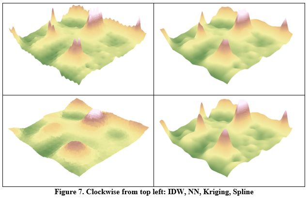
Based on the results from each of the interpolation
methods used compared to the actual sandbox where topographic data was
collected, it appears that the Spline method produced the best
representation of the real-world model. The reasons for this are that it is the
smoothest of the four spatial analysis interpolations methods used for this
example. The IDW method produced a pockmarked surface where each of the
locations where data was collected are visible. The Nearest Neighbor
method produced a surface very close to the Spline method but there was
still a small amount of jaggedness present near some of the larger jumps in
elevation. Finally, the Kriging method
did produce a surface model that was less vertically exaggerated but was still
jagged in many ways and did not represent the smoothness present in the real-world
model.
Conclusion
At
the end of this lab exercise, myself and my lab partners had gained valuable experience
in collecting and analyzing topographical data. Of the many interpolation
methods that we employed to convert our collected data to a 3D surface, some specific
methods ended up working better than others, with the Spline method outputting
the best surface model that was the most similar to the real world sandbox model.
The various skills that I have gained through the course of this lab exercise
will be valuable both in my future education and in my future geographic
exploits.
No comments:
Post a Comment